So far every demo has had a single neuron: one weight, one bias, one activation function. Once you start connecting neurons together, something interesting happens, the combined output can model shapes that no single neuron ever could.
Chaining neurons (depth)
Take two ReLU neurons in series. The first neuron transforms the input with its weight and bias, then applies ReLU. The second neuron takes that output as its input, applies its own weight and bias, then applies ReLU again. Drawn with the notation from the last part, the chain looks like this:
h becomes the second neuron's input; each neuron has its own weight on its incoming connection and its own bias from below. Data only ever flows left to right.The second neuron doesn't see the original input. It sees whatever the first neuron decided to pass on. As you tune the weight and bias of the second neuron, you are reshaping a signal that has already been non-linearised. The combined result can look like a clipped ramp, a shifted step, or other shapes that neither neuron could produce alone.
Follow some actual numbers through the chain to see this happen. Set w1 = 1, b1 = 0 on the first neuron and w2 = 1, b2 = -1 on the second (the same values the demo below starts with), and trace each input through all four steps:
| x | z1 = 1·x + 0 | h = ReLU(z1) | z2 = 1·h - 1 | y = ReLU(z2) |
|---|---|---|---|---|
| -2 | -2 | 0 | -1 | 0 |
| -1 | -1 | 0 | -1 | 0 |
| 0 | 0 | 0 | -1 | 0 |
| 1 | 1 | 1 | 0 | 0 |
| 2 | 2 | 2 | 1 | 1 |
| 3 | 3 | 3 | 2 | 2 |
Read the columns left to right and you can watch each neuron take its turn. The first neuron silences everything below x = 0 (the h column). The second neuron then subtracts 1 and silences anything that remains below that bar, so the output stays at zero all the way up to x = 1 and only then starts to rise.
To be clear about what is and is not remarkable here: a single neuron could produce this particular ramp perfectly well, ReLU(x − 1) switches on at 1 in one step. What the chain demonstrates is not a new shape but a new behaviour: the second neuron never saw x at all. It was handed h, and applied its own threshold to that. The two cutoffs compose, and the first neuron's decision changes what the second one is deciding about.
That is the property worth having, and the demo below lets you find shapes where it genuinely pays off.
Try it: two ReLU neurons in series
The dashed line below is the first neuron's output, h = ReLU(w1·x + b1). The solid dark-red line is the final output after the second neuron, y = ReLU(w2·h + b2). Tune all four knobs and watch the second neuron reshape what the first one hands it.
y = ReLU(1.00 · ReLU(1.00x + 0.00) + -1.00)
Some shapes to hunt for. With the default settings the second neuron delays the first one's ramp: the output stays silent until the first neuron's signal is strong enough to clear b2. As noted above, one neuron could manage that shape too.
Now set w2 = -1, b2 = 1, and you get something a single ReLU genuinely cannot produce: a plateau that falls away to zero. Here the limit is structural rather than a matter of tuning, and the demo below lets you prove it to yourself.
Try to beat it with one neuron
The dashed green line is that falling plateau. Your job is to match it.
Start in One neuron mode, which gives you a single ReLU with four knobs, more freedom than a plain neuron: a weight and bias going in, and a scale and shift coming out. Slide them all you like, and watch the mismatch score. Then switch to Two neurons chained and set w2 = -1, b2 = 1.
However you tune the single neuron, the mismatch bottoms out around 0.0121 and will not go lower. (Press "Set the best values" to jump straight to that best attempt.) The two-neuron chain reaches exactly 0.
The reason is worth stating plainly, because it is the whole argument for depth: one ReLU has exactly one kink in it. Its output can only ever be flat-then-sloping or sloping-then-flat, one bend, whatever numbers you choose. The falling plateau has two bends, so it needs two kinks, so it needs two neurons. Each layer of depth buys another fold in the signal, and no amount of knob-turning on a single neuron substitutes for it.
Parallel neurons (specialisation)
Instead of chaining, put neurons in parallel. Each gets the same input but has its own weight and bias, its own private view of the input. Their outputs are summed to produce the final result:
x fans out to every neuron, each applies its own weight, bias, and ReLU, and the five results are added together into a single output.Now each neuron is free to focus on a different region of the input space. That phrase is doing most of the work in this article, so it is worth unpacking, and it turns out to fall straight out of the ReLU arithmetic rather than being a metaphor.
A ReLU neuron computes w·xᵢ + b and then clips anything negative to zero. So for any given neuron there are only two kinds of input in the world:
- inputs where
w·xᵢ + bcomes out negative: the neuron outputs 0 and contributes nothing at all to the sum - inputs where
w·xᵢ + bcomes out positive: the neuron outputs a sloped line and contributes
The boundary between the two sits exactly where w·xᵢ + b = 0, which is to say at xᵢ = −b/w. Everything on the active side of that point is the neuron's active region: the stretch of inputs it actually has an opinion about. Outside it the neuron is silent, and whatever the network answers there is being decided entirely by its colleagues.
Here are the three neurons the demo below starts with, read that way:
| Neuron | Switch-on point (−b/w) | Active region | Silent for |
|---|---|---|---|
w = 1, b = −1 |
x = 1 | x > 1 | x < 1 |
w = −1, b = −1 |
x = −1 | x < −1 | x > −1 |
w = 0.5, b = 0 |
x = 0 | x > 0 | x < 0 |
Read down the table and the division of labour appears on its own. Below −1, only the second neuron is speaking. Between −1 and 0, all three are silent and the sum is flat zero. Between 0 and 1, only the third contributes. Above 1, the first and third are both on and their slopes add together. Four stretches of input, each handled by a different combination of neurons, and the handover from one stretch to the next is exactly where a bend appears in the total curve.
Two things follow from this. First, it explains why the sum comes out as straight segments joined at kinks rather than a genuinely smooth curve: within any one stretch the same fixed set of neurons is switched on, each of them linear, so their sum is linear too. The shape can only change where a neuron flips on or off. Second, nobody hands out these assignments. A neuron's switch-on point is −b/w, built from its own two knobs, so every time gradient descent nudges w or b it is also sliding that boundary along. The specialisation is not designed by anyone, it is a by-product of minimising the loss.
For the curious: the stretch of inputs where a neuron is switched on is usually called its active region, and the on/off pattern across the whole layer for a given input is that input's activation pattern. You will also meet the term activation space, which is related but is not the same thing: it means the space of the neurons' output values, one axis per neuron, rather than a slice of the input. Every input
xfed to the five-neuron layer pictured above lands somewhere in a five-dimensional activation space, and which corner of that space it lands in, which neurons are on and which are silent, is precisely what picks out its region of the input. The two are two views of the same fact, which is why the terms get used loosely, and in a deep network they blur together entirely: the "input space" that the third layer carves into regions is the second layer's activation space.
When you sum the neurons together, then, you are stitching together several local linear approximations, each one responsible for its own stretch of the input, into a single curve.
Try it: three ReLU neurons in parallel
Each thin coloured line below is one neuron's output; the thick dark-red line is their sum. Because every ReLU neuron contributes a hockey-stick that switches on at its own spot (set by its bias) and rises at its own rate (set by its weight), each knob you turn reshapes one bend of the total curve while the others stay put. That is the coordination trick in miniature: no neuron knows about the others, no one is in charge, yet the sum is a shape none of them could make alone, each neuron simply handles its own part of the problem.
Slide neuron 2's bias around and watch only the left side of the sum move; neuron 1's knobs own the right side, and neuron 3 tilts the middle. Every neuron minds its own patch of the input, and the network's answer is simply everyone's contributions added up. Scale this idea from three neurons to millions and you have the working principle of every neural network: lots of simple parts, each specialised on a fragment of the problem, coordinated by nothing more than addition.
This is specialisation, neurons carving up a problem into smaller sub-problems, each handling one piece. VGGNet, a famous image classification system, uses exactly this idea: early neurons look at tiny patches of pixels, and later layers combine those local features into global understanding.
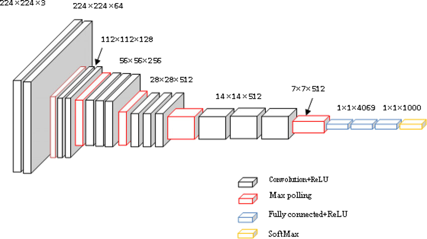
Demo 1: five neurons specialising on regions
The demo below has five neurons with fixed activation regions. Each neuron handles a different slice of the x-axis. Their summed output tries to approximate sin(x). Adjust the sliders to see how each neuron's weight and bias contributes to (or breaks) the overall fit.
Neurons are pre-assigned to x regions: N1 (x < −1.5) · N2 (−1.5 to −0.2) · N3 (−0.2 to 1) · N4 (1 to 2) · N5 (x ≥ 2)
Notice how changing one neuron's weight or bias only shifts that neuron's region of the output curve. Each neuron owns its slice.
Demo 2: gradient descent training a mini neural network
Now let gradient descent find the weights and biases automatically. The network below has 5 parallel neurons (each with its own weight and bias) feeding into a single output neuron that combines their signals. A group of neurons sitting side by side like this is called a layer; because this layer sits between the input and the output, hidden from both, it is called a hidden layer. The goal: approximate sin(x).
Press Train to run gradient descent. You can adjust the number of iterations and learning rate before training. Press Reset to start over with new random weights.
What to explore
- Press Train multiple times (after Reset), because weights are initialised randomly, you will get different results each time. Some runs converge faster, some get stuck.
- Try 3 neurons vs 12 neurons: more neurons give the model more capacity to approximate the sine curve. Fewer neurons means a coarser approximation.
- Adjust the learning rate: try 0.005 (slow), 0.05 (good), and 0.2 (may diverge).
- Try 50,000 iterations: the model keeps improving as long as training continues.
- Look closely at the fitted curve: every hidden neuron here uses ReLU, so the "smooth" fit is really many straight-line pieces stitched together. With 3 neurons the kinks are easy to spot; with 12 they blur into an apparently smooth wave.
The broader picture
What you just saw, a tiny network with a hidden layer learning to approximate a function, is the same fundamental mechanism behind all modern neural networks. ChatGPT, image classifiers, recommendation engines: they are all doing the same thing at a larger scale.
- Width (more neurons in a layer) gives the model more capacity to specialise.
- Depth (more layers) lets the model learn hierarchical features.
- This arrangement, neurons in layers with signals flowing strictly one way, has a proper name: a feedforward neural network, the most fundamental of all network architectures. It gets a full introduction of its own as the opening part of the LLM Basics series.
- Gradient descent finds the weights and biases.
- The loss function tells it how well it is doing.
This is also the moment to pay off a term that has been hovering since the training-loop diagram in Part 5: backpropagation. With one neuron, working out each parameter's slope was a single formula. In a network, a hidden neuron affects the loss only through the neurons after it, so to know how much w1 mattered, you first have to know how much the output it fed into mattered. Backpropagation is simply the bookkeeping that works this out efficiently: start from the error at the output and pass responsibility backwards through the network, layer by layer, so every weight and bias learns its own share of the blame. That is exactly what the training demo above is doing on every step. The result is the same gradient descent you already know, just with the slopes computed in reverse order.
Everything you have learned in this series, weights, biases, loss functions, gradient descent, learning rate, generalisation, local minima, activation functions, neurons, is operating inside every model you use.
Next: From Straight Lines to ChatGPT: the series opened with "LLMs are just predicting the next token." Time to close the loop and see how everything you have learned scales up to a language model.